
The clustered heatmap: reading samples × variables at a glance
A heatmap shows a whole table at once: one row per sample, one column per measured variable, and the value in each cell drawn as a colour. On its own that is just a coloured table. What makes it a tool is the clustering: the rows are reordered so that samples with similar profiles sit together, the columns so that variables that rise and fall together sit together, and the two trees drawn alongside show how those groupings formed. Blocks of one colour along the diagonal are the structure in your data.
The data
Twelve bread samples in three formulations (four loaves each) and five measurements per loaf — samples down the rows, variables across, with the formulation as the group:
| Sample | Moisture (%) | Hardness (N) | Volume (mL) | Crumb L* | Panel score |
|---|---|---|---|---|---|
| Control 1 | 38.2 | 4.1 | 1620 | 72.4 | 6.8 |
| Control 2 | 37.9 | 4.4 | 1590 | 71.8 | 6.5 |
| Control 3 | 38.5 | 3.9 | 1650 | 72.9 | 7.0 |
| Control 4 | 38.0 | 4.2 | 1610 | 72.1 | 6.7 |
| +Fibre 1 | 40.8 | 6.3 | 1380 | 64.2 | 5.4 |
| +Fibre 2 | 41.2 | 6.8 | 1350 | 63.5 | 5.1 |
| +Fibre 3 | 40.5 | 6.1 | 1400 | 64.8 | 5.6 |
| +Fibre 4 | 41.0 | 6.5 | 1370 | 63.9 | 5.3 |
| +Protein 1 | 36.4 | 5.2 | 1480 | 68.9 | 6.1 |
| +Protein 2 | 36.1 | 5.6 | 1450 | 68.2 | 5.9 |
| +Protein 3 | 36.7 | 5.0 | 1500 | 69.3 | 6.3 |
| +Protein 4 | 36.3 | 5.4 | 1470 | 68.6 | 6.0 |
Matrix layout with a group column: MinutePlot draws the coloured strip beside the rows from it.
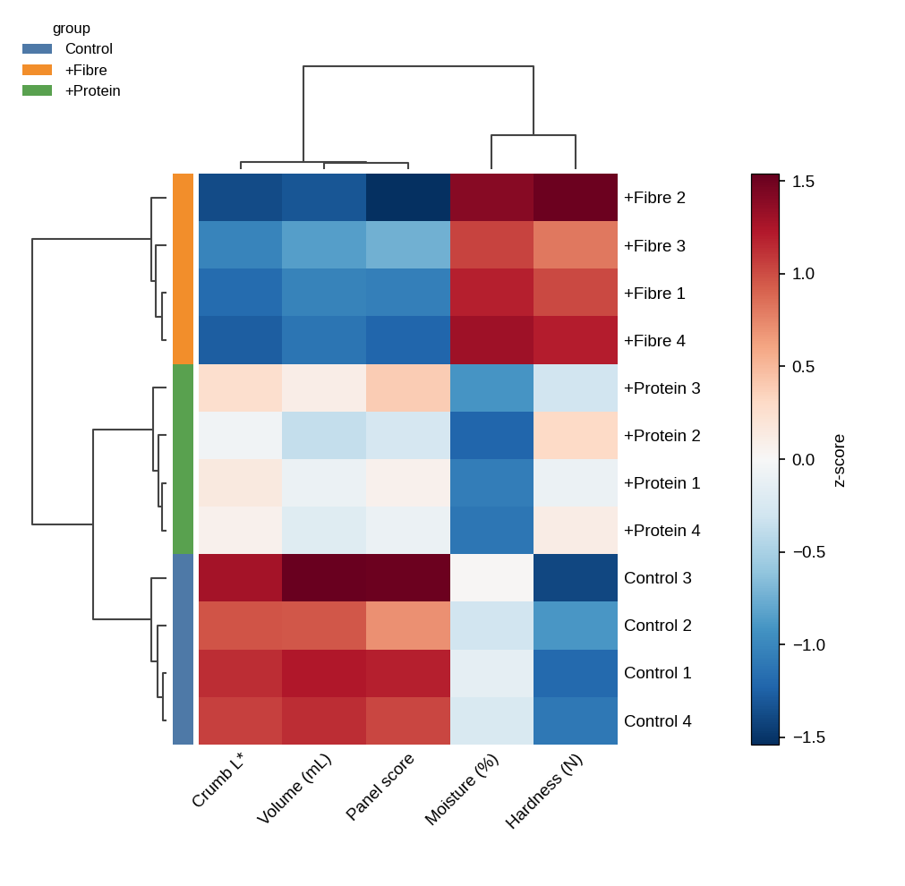
The figure MinutePlot produces from this table: z-scores as colours, samples and variables reordered by their trees, the formulation strip beside the rows — the three formulations fall into three blocks.
The z-scores
Variables come in different units — a percentage, a hardness, a count — so the values are first standardised per variable: each column is shifted to mean 0 and scaled to standard deviation 1. A cell then says how many standard deviations that sample lies above (red) or below (blue) that variable’s own mean: 0 is the mean, ±1 ordinary, ±2 or more unusual. Because every column is on the same scale, colours can be compared across the whole picture; the raw-value option keeps the original units and is only sensible when every column shares them.
The two trees
Each tree is a hierarchical clustering (Ward, 1963, by default): starting from single samples (or variables), the two closest are joined, then the next closest, until one tree remains. The height at which two branches join is their distance on the standardised table — samples that join low are alike, a long stem before a join means the branches differ a lot. The order table under the figure lists, for each entry, the height at which it joins the next one: a small number means the two are alike, a large one means a real division of the tree runs between them. It is a reading aid for the picture, not a result to report.
When to use it, and when PCA
The heatmap keeps every variable visible and answers “which samples resemble which, and on which variables?” directly. PCA (Pearson, 1901) compresses the same table into a few components and answers “what are the main directions of variation?” The two are complementary: the heatmap for the detail, the score plot for the overview. With a group column, the strip beside the rows shows whether the clustering rediscovers your groups — which is a useful sanity check before any hypothesis test.
Reporting it
State that values were standardised per variable, the linkage (Ward) and distance (Euclidean), and that both samples and variables were clustered; then describe the blocks you see, naming the samples and the variables that define them. Say which tree is on or off if you switched one off for the figure.
- Ward, J. H. (1963). Hierarchical grouping to optimize an objective function. Journal of the American Statistical Association, 58(301), 236–244. https://doi.org/10.1080/01621459.1963.10500845
- Pearson, K. (1901). On lines and planes of closest fit to systems of points in space. The London, Edinburgh, and Dublin Philosophical Magazine and Journal of Science, 2(11), 559–572. https://doi.org/10.1080/14786440109462720