
Independent t-test: a worked example
The independent (unpaired) t-test answers the simplest experimental question there is: do these two groups differ? It goes back to Student’s 1908 paper written at the Guinness brewery, and it remains the right first tool whenever two separate groups of subjects are measured once each.
The data
Root mass (g) of plants grown with and without a growth treatment, eight plants per group:
| Values | ||||||||
|---|---|---|---|---|---|---|---|---|
| r1 | r2 | r3 | r4 | r5 | r6 | r7 | r8 | |
| Control | 5.1 | 5.4 | 4.9 | 5.6 | 5.0 | 5.3 | 4.8 | 5.2 |
| Treated | 6.0 | 6.4 | 5.8 | 6.6 | 6.1 | 5.9 | 6.3 | 6.2 |
r = replicate: r1 is replicate 1, r2 replicate 2, and so on.
Laid out exactly as MinutePlot’s data grid for a two-group comparison: one row per group, one column per replicate.
Check the assumptions first
Two things must hold, approximately: each group’s values are normally distributed (checked with the Shapiro–Wilk test), and the two groups have similar spread. Here both groups have a standard deviation of 0.27 g — as similar as it gets. When variances differ clearly, use Welch’s version of the test, which drops the equal-variance assumption; MinutePlot switches automatically when the data call for it.
Why Welch, and only Welch. MinutePlot performs Welch’s t-test, which does not assume equal variances and is the modern recommended default — and R’s own default in t.test(); the Student equal-variance variant is intentionally not offered. Readers comparing with tools that default to Student’s test (SPSS, Excel) may see small differences in t and p for that reason alone — the validation page shows both side by side.
The result
Control mean 5.16 ± 0.27 g; treated mean 6.16 ± 0.27 g. The test gives t(14) = 7.49, p < 0.001, with a very large effect size (Cohen’s d = 3.7). The treatment increased root mass by about 1.0 g — roughly 19% — and the difference is far too large to be sampling noise.
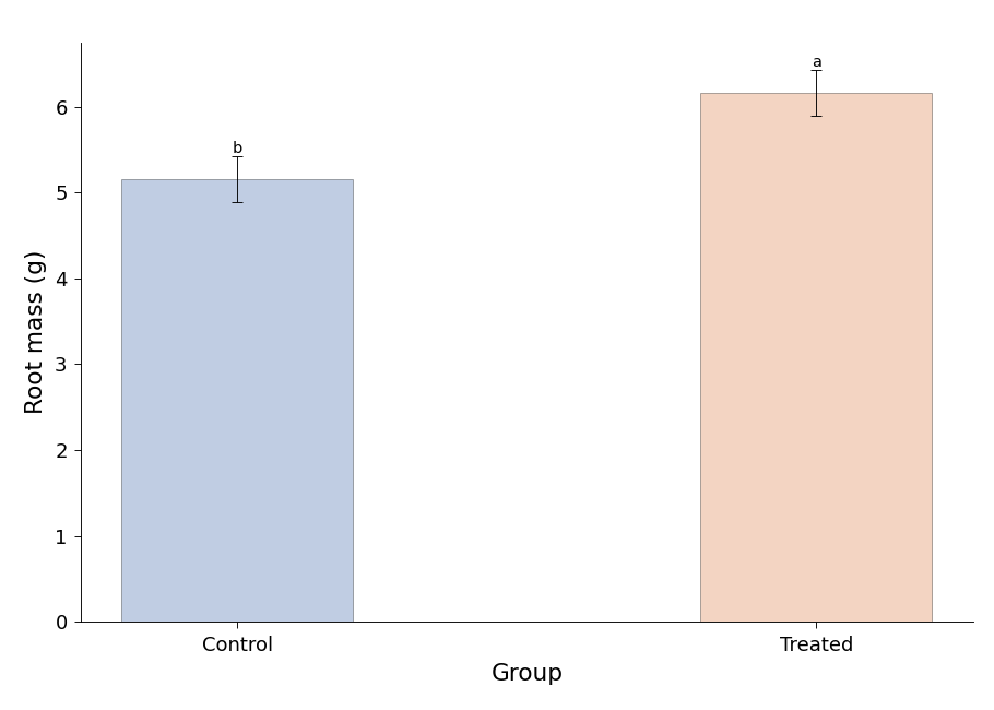
The figure MinutePlot produces for this analysis: group means with error bars, and letters marking the significant difference.
Styling and exporting this figure: see Figure styling and Exporting & downloading.
Report it like this
“Treated plants produced greater root mass than controls (5.16 ± 0.27 g vs. 6.16 ± 0.27 g; independent t-test, t(14) = 7.49, p < 0.001).”
Common pitfalls
Do not use this test when the same subjects appear in both columns (that is the paired t-test), and do not run several t-tests to compare three or more groups — that inflates false positives; use one-way ANOVA instead.
- Student (1908). The probable error of a mean. Biometrika, 6(1), 1–25. https://doi.org/10.1093/biomet/6.1.1
- Shapiro, S. S., & Wilk, M. B. (1965). An analysis of variance test for normality (complete samples). Biometrika, 52(3–4), 591–611. https://doi.org/10.1093/biomet/52.3-4.591
- Montgomery, D. C. (2017). Design and Analysis of Experiments (9th ed.). John Wiley & Sons.