
Binary logistic regression: predicting yes / no outcomes
An outcome that is one of two things — a seed germinates or not, a sample passes or fails — cannot be fitted with ordinary regression: the answer is a probability, bounded by 0 and 1. Logistic regression models the log-odds of the outcome as a linear function of the predictors, so each coefficient says how the odds change per unit of that predictor.
The data
One row per observation: the outcome as 0 / 1, then the predictors (here the classic mtcars question: is a car’s transmission manual, from its weight and horsepower?):
| Car | am | wt | hp |
|---|---|---|---|
| Mazda RX4 | 1 | 2.620 | 110 |
| Datsun 710 | 1 | 2.320 | 93 |
| Hornet 4 Drive | 0 | 3.215 | 110 |
| … | … | … | … |
| Volvo 142E | 1 | 2.780 | 109 |
Logistic layout: the 0 / 1 outcome column, then one column per predictor; 32 rows in the full dataset.
In MinutePlot
Choose Binary logistic regression, mark the outcome column, run. The table gives each coefficient on the log-odds scale with its standard error, z and p, plus the odds ratio with its confidence interval; the fit summary reports the deviances, AIC, McFadden’s pseudo-R² and the likelihood-ratio test of the whole model.
The result
Weight: −8.08 log-odds per 1000 lb (p = 0.008) — heavier cars are far less likely to be manual; horsepower: +0.036 per hp (p = 0.041). Residual deviance 10.1 against a null deviance of 43.2: the two predictors explain most of the pattern (McFadden R² = 0.77).
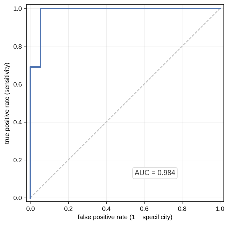
The figure MinutePlot produces for a model with more than one predictor: the ROC curve with its AUC (a single-predictor model shows the probability curve instead).
Styling and exporting this figure: see Figure styling and Exporting & downloading.
Report it like this
“The odds of a manual transmission fell with weight (β = −8.08, p = 0.008) and rose with horsepower (β = 0.036, p = 0.041); logistic regression, likelihood-ratio test p < 0.001.”
- Hosmer, D. W., Lemeshow, S. & Sturdivant, R. X. (2013). Applied Logistic Regression, 3rd ed. Wiley.